
2D Dispersive Transport in a Uniform Flow Field (aligned)#
Capabilities Tested#
This two-dimensional transport problem — with a constant rate mass loading point source in a steady-state flow field — tests the Amanzi flow process kernel as well as advection and dispersion features of the transport process kernel. Capabilities tested include:
single-phase, one-dimensional flow
two-dimensional transport
steady-state saturated flow
constant-rate solute mass injection well
advective transport
dispersive transport
longitudinal and transverse dispersivity
non-reactive (conservative) solute
homogeneous porous medium
isotropic porous medium
statically refined (non-uniform) mesh
For details on this test, see About.
Background#
This test problem is motivated by confined flow applications with transport from a relatively small source. A typical source would be a well that is fully screened over the confined flow interval. In this case, the steady-state flow field is uniform and the injection well tracer mass source rate does not affect the flow field. The dominant transport processes are advection and dispersion. Dispersion results in the spreading of the released mass in all directions, including upstream of the source location. Longitudinal dispersivity (in the axis of flow) is typically up to an order of magnitude larger than the transverse dispersivity. Accuracy of the simulated concentrations in the vicinity of the source is sensitive to the resolution of the grid and the numerical transport scheme.
The analytical solution uses Green’s functions to integrate solutions for point and line sources in each of the principle coordinate directions to generate advective-dispersive transport from a point, line, planar, or rectangular sources. The verification data used in this test is generated from AT123D, a program of these analytical solutions for one-, two-, or three-dimensional transport of heat, dissolved chemicals, or dissolved radionuclides in a homogeneous aquifer subject to a uniform, stationary regional flow field [Yeh81]. The assumption is that the modeled aquifer is infinite in the direction of flow but can be considered finite or infinite in the vertical and transverse horizontal directions. The test problem specification is described in Problem 5.2 of [Ale07]. The verification data from AT123D that is used to compare against Amanzi output is listed in Tables 5.2.3, 5.2.4, and 5.2.5 of that document.
Model#
The analytical solution addresses the advection-dispersion equation (saturation \(s_l = 1\)):
where \(\phi\) is porosity, \(C\) is the solute concentration [kg/m3], \(t\) is time [s], \(Q\) is solute mass injection rate [kg of tracer/m3/s], and \(\boldsymbol{D}\) is the dispersion tensor:
Let \(\boldsymbol{v} = (v_x,\,v_y)\) denote the pore velocity. Then, the diagonal entries in the dispersion tensor are
where \(\alpha_L\) is longitudinal dispersivity [m] and \(\alpha_T\) is transverse dispersivity [m]. The off-diagonal entries are:
Problem Specification#
Schematic#
The domain, flow direction, and source location are shown in the following schematic.
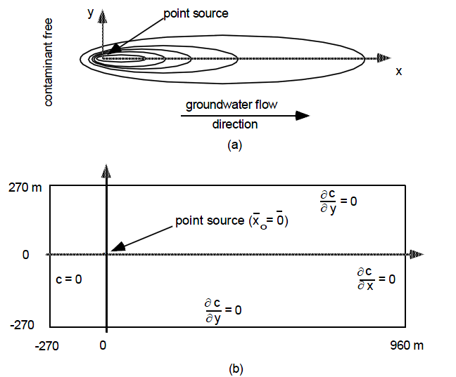
a) Plume from point source loading in a constant uniform groundwater flow field. b) Problem domain.#
Mesh#
The background mesh consists of square cells with size \(H=15\) m. It has 83 grid cells in the x-direction and 37 grid cells in the y-direction. The mesh is gradually refined toward the source such that the well is represented by a square cell of \(h=0.46875\) [m] (\(h = H/32\)). The mesh refinement adds 17% more cells.
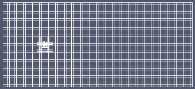
Computational mesh with 3650 cells and static refinement around the well.#
Variables#
initial concentration condition: \(C(x,0)=0 \: \text{[kg/m}^3\text{]}\)
constant solute mass injection rate: \(Q=8.1483 \times 10^{-8} \: \text{[kg/m}^3\text{/s]}\)
volumetric fluid flux: \(\boldsymbol{q}=(1.8634 \times 10^{-6},\,0.0) \: \text{[m}^3 \text{/(m}^2 \text{ s)]}\) or \(\text{[m/s]}\)
Material properties:
isotropic hydraulic conductivity: \(K = 84.41 \: \text{[m/d]}\)
derived from: \(K=\frac{k \rho g}{\mu}\), where permeability, \(k = 10^{-10} \text{ [m}^2\text{]}\)
porosity: \(\phi=0.35\)
longitudinal dispersivity: \(\alpha_L=21.3 \: \text{[m]}\)
transverse dispersivity: \(\alpha_T=4.3 \: \text{[m]}\)
fluid density: \(\rho = 998.2 \: \text{[kg/m}^3\text{]}\)
dynamic viscosity: \(\mu = 1.002 \times 10^{-3} \: \text{[Pa} \cdot \text{s]}\)
gravitational acceleration: \(g = 9.807 \: \text{[m/s}^2\text{]}\)
total simulation time: \(t=1400 \: \text{[d]}\)
Results and Comparison#
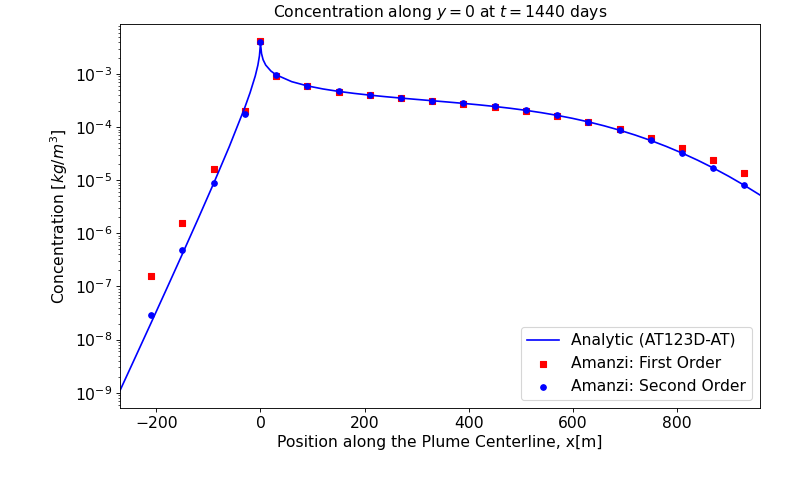
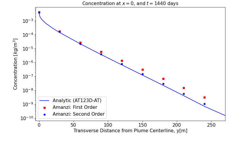
The plume structure is characterized by three line cuts. The first cut is given by line \(y=0\) that goes through the well. The two other cuts are given by lines \(x=0\) and \(x=424\).
(Source code, png, hires.png, pdf)
x [m] |
Analytic (AT123D-AT) |
Amanzi First-Order |
Amanzi Second-Order |
|---|---|---|---|
-210.0 |
2.08846e-08 |
1.58878e-07 |
2.88735e-08 |
-150.0 |
4.10954e-07 |
1.56474e-06 |
4.90770e-07 |
-90.0 |
8.72377e-06 |
1.64614e-05 |
8.91355e-06 |
-30.0 |
2.35916e-04 |
1.99727e-04 |
1.76350e-04 |
0.0 |
3.77529e-03 |
4.09233e-03 |
3.99032e-03 |
30.0 |
9.64773e-04 |
9.32631e-04 |
9.49716e-04 |
90.0 |
5.96679e-04 |
5.85850e-04 |
5.91764e-04 |
150.0 |
4.70106e-04 |
4.67129e-04 |
4.69614e-04 |
210.0 |
3.99571e-04 |
3.97253e-04 |
3.99730e-04 |
270.0 |
3.51580e-04 |
3.48273e-04 |
3.51877e-04 |
330.0 |
3.13736e-04 |
3.08766e-04 |
3.14063e-04 |
390.0 |
2.79428e-04 |
2.72836e-04 |
2.79776e-04 |
450.0 |
2.44507e-04 |
2.37203e-04 |
2.44893e-04 |
510.0 |
2.06811e-04 |
2.00467e-04 |
2.07238e-04 |
570.0 |
1.66406e-04 |
1.62878e-04 |
1.66836e-04 |
630.0 |
1.25510e-04 |
1.25992e-04 |
1.25874e-04 |
690.0 |
8.76140e-05 |
9.20266e-05 |
8.78410e-05 |
750.0 |
5.60091e-05 |
6.30470e-05 |
5.60759e-05 |
810.0 |
3.25149e-05 |
4.03001e-05 |
3.24525e-05 |
870.0 |
1.70276e-05 |
2.39574e-05 |
1.69049e-05 |
930.0 |
8.00226e-06 |
1.35531e-05 |
7.98544e-06 |
The analytic data were computed with the AT123DAT software package. A difference is observed near the downstream boundary for Amanzi with the first-order transport scheme (boxes), while the second-order transport scheme provides excellent match (circles).
(Source code, png, hires.png, pdf)
y [m] |
Analytic (AT123D-AT) |
Amanzi First-Order |
Amanzi Second-Order |
|---|---|---|---|
0.0 |
3.77529e-03 |
4.09233e-03 |
3.99032e-03 |
30.0 |
1.42512e-04 |
1.75114e-04 |
1.66302e-04 |
60.0 |
2.16132e-05 |
2.68345e-05 |
2.15528e-05 |
90.0 |
3.71210e-06 |
5.94555e-06 |
4.04684e-06 |
120.0 |
6.69535e-07 |
1.34177e-06 |
7.74937e-07 |
150.0 |
1.23023e-07 |
3.04949e-07 |
1.51144e-07 |
180.0 |
2.25231e-08 |
6.82272e-08 |
2.94816e-08 |
210.0 |
4.02061e-09 |
1.47356e-08 |
5.65434e-09 |
240.0 |
6.89736e-10 |
3.05866e-09 |
1.05997e-09 |
(Source code, png, hires.png, pdf)
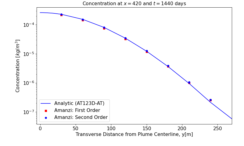
y [m] |
Analytic (AT123D-AT) |
Amanzi First-Order |
Amanzi Second-Order |
|---|---|---|---|
30.0 |
2.28980e-04 |
2.20580e-04 |
2.28331e-04 |
60.0 |
1.53780e-04 |
1.45459e-04 |
1.52472e-04 |
90.0 |
8.11670e-05 |
7.58302e-05 |
8.04473e-05 |
120.0 |
3.46429e-05 |
3.24695e-05 |
3.47067e-05 |
150.0 |
1.22755e-05 |
1.17784e-05 |
1.25957e-05 |
180.0 |
3.68637e-06 |
3.69969e-06 |
3.93498e-06 |
210.0 |
9.51336e-07 |
1.02136e-06 |
1.07585e-06 |
240.0 |
2.15023e-07 |
2.54050e-07 |
2.64209e-07 |
References#
S. Aleman. Porflow testing and verification. Technical Report, Savannah River National Laboratory, 2007.
G. T. Yeh. At123d: analytical transient one-, two-, and three-dimensional simulation of transport in the aquifer system. Technical Report, Oak Ridge National Laboratory, Oak Ridge, TN, 1981.
About#
Directory: testing/verification/transport/saturated/steady-state/dispersion_aligned_point_2d
Authors: Konstantin Lipnikov, Marc Day, David Moulton, Steve Yabusaki
Maintainer(s): Konstantin Lipnikov, Marc Day
Input Files:
amanzi_dispersion_aligned_point_2d-u.xml, Spec Version 2.3
mesh is amanzi_dispersion_aligned_point_2d.exo
Analytic solution computed with AT123D-AT
Subdirectory: at123d-at
Input Files:
at123d-at_centerline.list, at123d-at_centerline.in
at123d-at_slice_x=0.list, at123d-at_slice_x=0.in,
at123d-at_slice_x=420.list, at123d-at_slice_x=420.in
Todo
Documentation:
Do we need a short discussion on numerical methods (i.e., discretization, splitting, solvers)?
Store Gold Standard simulation results (need name and location)?
Add plots for structured AMR results to these plots or make subplots
What about colormap plot of the field?
Schematics should include citation
Schematics should be redone with tikz.
Citations may/should be improved with the natbib extension for sphinx?
Tables need to be centered and captions added (more sphinx tuning/extensions)
Results from Structured AMR mesh infrastructure runs need to be added.
Should we separate authors/maintainers into code and documentation?