
Transient Flow in a 2D Confined Aquifer with a Linear Strip#
Capabilities Tested#
This two-dimensional flow problem — with a constant pumping rate in a heterogeneous confined aquifer — tests the Amanzi saturated flow process kernel. Capabilities tested include:
single-phase, two-dimensional flow
transient flow
saturated flow
constant-rate pumping well
constant-head (Dirichlet) boundary conditions
heterogeneous isotropic porous medium
uniform mesh
For details on this test, see About.
Background#
Butler and Liu (1991) [BL91] developed a semi-analytical solution for calculating drawdown in an aquifer system, in which an infinite linear strip of one material is embedded in a matrix of different hydraulic properties. The problem is interested in the drawdown as a function of location and time due to pumping from a fully penetrating well located in any of three zones. The problem is solved analytically in the Fourier-Laplace space and the drawdown is solved numerically by inversion from the Fourier-Laplace space to the real space.
The solution reveals several interesting features of flow in this configuration dependening on the relative contrast in material transmissivity. If the transmissivity of the strip is much higher than that of the matrix, linear and bilinear flow regimes dominate during the pumping test. If the contrast between matrix and strip properties is not as extreme, radial flow dominates.
Model#
Flow within zones that do not contain the pumping well can be described mathematically in terms of drawdown \(s\) as (1)
where \(s_i\) is the drawdown [L] in material \(i\), \(t\) is time [T], \(T_i\) is the transmissivity [L2/T] of material \(i\), and \(S_i\) is the storage coefficient [-] of material \(i\).
Flow within zones that contain the pumping well can be represented as
where \(Q\) is the pumping rate [L3/T] from well located at \((a,b)\), \(\delta(x)\) is the Direc delta function, being 1 for \(x = 0\) and \(0 \text{ otherwise}\).
The initial conditions are the same for all three zones:
The boundary conditions are:
Problem Specification#
Schematic#
The domain configuration and well locations are indicated in the following schematic. The origin of the coordinate system is shown in the figure as ‘o’.
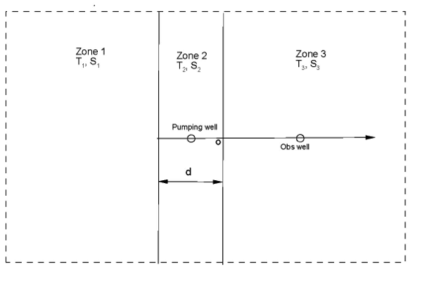
Schematic of the Butler and Liu’s Linear Strip verification problem.#
Mesh#
The background mesh is \(1202 \: m \times 1202 \: m \times 1 \: m\) and consists of 361,201 cells. There are 601 cells in the x-direction, 601 cells in the y-direction, and 1 cell in the z-direction.
Variables#
Domain:
\(x_{min} = y_{min} = 1202, z_{min} = 0 \text{ [m]}\)
\(x_{max} = y_{max} = 1202, z_{max} = 1 \text{ [m]}\)
aquifer thickness: \(b=z_{max}-z_{min} = 1 \text{ [m]}\)
Zone 1 (left zone):
\(-1202 \leq x \leq -10\)
\(-1202 \leq y \leq 1202\)
\(0 \leq z \leq 1\)
Zone 2 (strip):
\(-10 \leq x \leq 10\)
\(-1202 \leq y \leq 1202\)
\(0 \leq z \leq 1\)
Zone 3 (right zone):
\(10 \leq x \leq 1202\)
\(-1202 \leq y \leq 1202\)
\(0 \leq z \leq 1\)
pumping well location: \((a,b) = (0,0) \text{ [m]}\)
observation well locations:
\((x_{obs24},y_{obs24},z_{obs24}) = (24,0,1) \text{ [m]}\)
\((x_{obs100},y_{obs100},z_{obs100}) = (100,0,1) \text{ [m]}\)
Boundary and initial conditions:
initial condition: \(s(x,y,0)=0 \text{ [m]}\)
constant-head (Dirichlet) boundary conditions: \(s(x_{min,max},y_{min,max},t) = 0 \text{ [m]}\)
well-head pumping rate: \(Q = -11.5485 \text{ [m}^3 \text{/s]} = 1000 \text{ [m}^3 \text{/d]}\)
duration of pumping: \(t_{max} = 31.7 \text{ [yrs]}\)
Material properties:
transmissivity (all isotropic):
\(T_1 = 0.11574 \text{ [m}^2 \text{/s]}\)
\(T_2 = 0.011574 \text{ [m}^2 \text{/s]}\)
\(T_3 = 0.0011574 \text{ [m}^2 \text{/s]}\)
derived from: \(T=Kb\), where \(K=\frac{k \rho g}{\mu}\)
intrinsic permeability: \(k_1 = 1.187 \times 10^{-8}, k_2 = 1.187 \times 10^{-9}, k_3 = 1.187 \times 10^{-10} \text{ [m}^2 \text{]}\)
storativity:
\(S_1=5.0 \times 10^{-3} \: \text{[-]}\)
\(S_2=2.0 \times 10^{-3} \: \text{[-]}\)
\(S_3=2.0 \times 10^{-4} \: \text{[-]}\)
derived from: \(S=S_s b\), where \(b=10 \: \text{[m]}\)
porosity: \(\phi_{1,2,3} = 0.25\)
fluid density: \(\rho = 1000.0 \: \text{[kg/m}^3\text{]}\)
dynamic viscosity: \(\mu = 1.002 \times 10^{-3} \: \text{[Pa} \cdot \text{s]}\)
gravitational acceleration: \(g = 9.807 \: \text{[m/s}^2\text{]}\)
Results and Comparison#
(Source code, png, hires.png, pdf)
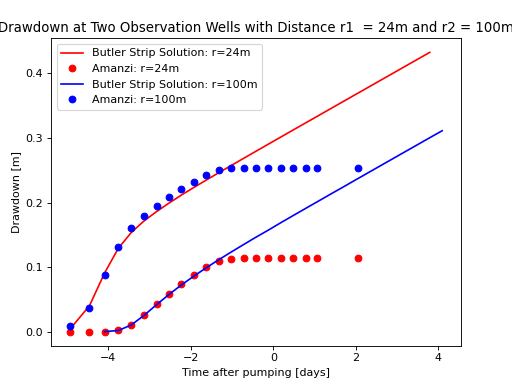
The comparison shows that the results from the Amanzi model match the analytical solution very well at early time, and that they deviate when the effect of pumping hits the constant head boundary of the domain. Note that the analytical solution was developed for unbounded domain, so it is therefore expected that the two solutions will deviate from each other at late time. To show that such a deviation is indeed caused by the boundary effect, we also conducted numerical simulations using FEHM, a widely used numerical simulator for simulating heat and mass flow in subsurface environment [ZRDT97]. It is showed that the results from Amanzi are almost the same as those from FEHM, see [LHB14] for detailed comparison.
References#
J. J. Butler and W. Liu. Pumping test in non-uniform aquifers – the linear strip case. J. Hydrol., 128:69–99, 1991.
Z. Lu, D. Harp, and K. Birdsell. Comparison of the amanzi model against analytical solutions and the fehm model. Technical Report, Los Alamos National Laboratory, Los Alamos, NM, 2014.
G. A. Zyvoloski, B. A. Robinson, Z. V. Dash, and L. L. Trease. Summary of the models and methods for the fehm application-a finite-element heat-and mass-transfer code. Technical Report, Los Alamos National Laboratory, Los Alamos, NM, 1997.
About#
Directory: testing/verification/flow/saturated/transient/butler_strip_2d
Authors: Zhiming Lu (zhiming@lanl.gov), Dylan Harp (dharp@lanl.gov)
Maintainer(s): Zhiming Lu, Dylan Harp
Input Files:
amanzi_butler_strip_2d-u.xml
Spec: Version 2.3, unstructured mesh framework
Mesh: generated internally
Analytical Solutions
Directory: analytic/
Executable: butler_strip.x, compiled from FORTRAN code under the Linux environment.
Input Files:
now.dat
Output Files:
drdn.dat, drawdown as a function of time for all observation wells.
Todo
The analytical solution was solved using a FORTRAN code modified from the original code from Greg Ruskauf. We may need to implement the algorithm by ourselves or get permission from Greg Ruskauf for using the code. As the flow problem was solved analytically in the Laplace-Fourier transformed space, one needs to implement numerical inversion from the Laplace-Fourier transformed space back to the real space.