
Transient One-Dimensional Confined Flow to a Pumping Well (Theis)#
Capabilities Tested#
This transient one-dimensional (radial) flow problem tests the Amanzi saturated flow process kernel. Capabilities tested include:
single-phase, radial flow
transient, saturated flow
constant-rate pumping well (constant source term)
constant-head (Dirichlet) and no-flow boundary conditions
homogeneous porous medium
isotropic porous medium
uniform mesh
For details on this test, see About.
Background#
Groundwater resource evaluation is crucial to understanding the concept of groundwater yield. This concept is vital because it helps determine the maximum allowable pump rate out of an aquifer and the consequences on the water table. For example, pumping water out of the water table (unconfined aquifer) may dry up nearby wells due to the fall in the saturated thickness of the aquifer. This can be prevented by modeling the fall of the water table given a certain pumping rate.
To apply the analysis developed by Theis, three parameters must be known:
\(T\), transmissivity
\(S\), storativity
\(Q\), well-head pumping rate
Transmissivity [L2/T] of the aquifer is defined as:
where \(K\) is the hydraulic conductivity of the aquifer [L/T] and \(b\) is the saturated thickness of the aquifer [L]. Transmissivity values greater than 0.015 \(\frac{m^2}{s}\) represent aquifers capable of well exploitation. Storativity is a dimensionless parameter that describes the amount of water released by the aquifer per unit unit decline in hydraulic head in the aquifer, per unit area of the aquifer. Storativity can be calculated using:
where \(S_s\) is the specific storage [L-1], which describes the volume of water an aquifer releases from storage, per unit volume of aquifer, per unit decline in hydraulic head. For a confined aquifer, storativity is the vertically integrated specific storage value.
Lastly, the constant pumping rate, \(Q\), is the volume of water discharged from the well per unit time [L3/T].
Model#
Theis (1935) developed an analytical solution for transient (non- steady state) drawdown for a fully penetrating well by imposing the boundary conditions: \(h = h_0\) for \(t = 0\) and \(h \Rightarrow h_0\) as \(r \Rightarrow \infty\) [The35]. The equation assumes an infinite and uniform confined aquifer. When a well is pumped the water table declines toward the well and flow is induced toward the well from all directions. Theoretically, this flow can be idealized by purely radial symmetric flow and can be decribed by the equation below (this is analogous to heat flow by conduction developed by Fourier):
where \(h\) is hydraulic head [m], \(r\) is radial distance from the well [m], \(S\) is the aquifer storativity [-], \(T\) is the aquifer transmissivity [m2/s], \(Q\) is the volumetric pumping rate of the well [L3/T], and \(t\) is time [s]. Mathematically, \(Q\) is the point source.
The analytical solution of drawdown as a function of time and distance is found to be:
where
and
for which \(s\) is head drawdown [m], \(Q\) is the volumetric discharge rate of the well [L3/T], \(W(u)\) is the well function, and \(u\) is the argument of the well function. The integral approximation for the well function, W(u), for \(0 < u < 1\) is
and for \(u \geq 1\),
Note, \(W(u)\) can easily be determined from existing tables once \(u(r, t)\) is found which is a measure of aquifer response time. For a given value of t one can construct a draw down curve with respect to the distance from the pumping well, r.
Problem Specification#
Schematic#
Note, the values in the schematic correlate to the values found in Variables.
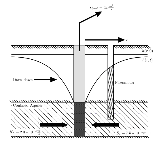
Illustration of transient drawdown in a confined aquifer.#
Mesh#
The mesh is generated in the input file. It consists of cells with size \(\Delta x=4\) m, \(\Delta y=4\) m, and \(\Delta z=10\) m. It has 600 grid cells in the x-direction and 600 grid cells in the y-direction, with a single cell in the z-direction.
Variables#
Domain:
\(x_{min} = y_{min} = z_{min} = -1200\) m
\(x_{max} = 1200\) m, \(y_{max} = 1200\) m, \(z_{max} = 10\) m
Boundary and initial conditions:
initial hydraulic head: \(h(r,0)=20.0 \: \text{[m]}\)
constant-head (Dirichlet) lateral boundary conditions: \(h(x_{max},t)=h(y_{max},t)=20.0 \: \text{[m]}\)
no-flow (Neumann) upper and lower boundary conditions
well-head pumping rate: \(Q=4.0 \: \text{[m}^3\text{/s]}\)
radial distance from well: \(r \: \text{[m]}\)
duration of pumping: \(t \: \text{[s]}\)
Material properties:
storativity: \(S=7.5 \times 10^{-4} \: \text{[-]}\), derived from \(S=S_s b\), where \(S_s=7.5 \times 10^{-5} \: \text{[m}^{-1} \text{]}\) and \(b=10 \: \text{[m]}\)
porosity: \(\phi = 0.2\)
transmissivity: \(T=4.7 \times 10^{-4} \: \text{[m}^2\text{/s]}\), derived from \(T=Kb\), where \(K=\frac{k \rho g}{\mu}\) and \(k = 2.35 \times 10^{-11} \: \text{[m}^2\text{]}\)
fluid density: \(\rho = 1000.0 \: \text{[kg/m}^3\text{]}\)
dynamic viscosity: \(\mu = 1.002 \times 10^{-3} \: \text{[Pa} \cdot \text{s]}\)
gravitational acceleration: \(g = 9.807 \: \text{[m/s}^2\text{]}\)
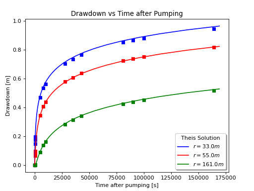
Results and Comparison#
(Source code, png, hires.png, pdf)
time [s] |
r [m] |
z [m] |
Analytic [m] |
Amanzi [m] |
0.0 |
55.0 |
5.0 |
0.0000000000 |
0.0000000002 |
0.0864 |
55.0 |
5.0 |
0.0000000000 |
0.0000000002 |
0.4 |
55.0 |
5.0 |
0.0000000000 |
0.0000000002 |
400.0 |
55.0 |
5.0 |
0.0608385188 |
0.0629942836 |
500.0 |
55.0 |
5.0 |
0.0786216376 |
0.0808372265 |
600.0 |
55.0 |
5.0 |
0.0947014814 |
0.0970139390 |
5000.0 |
55.0 |
5.0 |
0.3433506196 |
0.3453688505 |
8000.0 |
55.0 |
5.0 |
0.4058889734 |
0.4080982206 |
10000.0 |
55.0 |
5.0 |
0.4359300429 |
0.4382259416 |
28000.0 |
55.0 |
5.0 |
0.5762513445 |
0.5785810023 |
35000.0 |
55.0 |
5.0 |
0.6068911106 |
0.6092682000 |
43000.0 |
55.0 |
5.0 |
0.6351997488 |
0.6376562844 |
81000.0 |
55.0 |
5.0 |
0.7224685054 |
0.7246541630 |
90000.0 |
55.0 |
5.0 |
0.7370080987 |
0.7391540824 |
100000.0 |
55.0 |
5.0 |
0.7515518940 |
0.7535650703 |
164000.0 |
55.0 |
5.0 |
0.8198837286 |
0.8183153019 |
References#
C. V. Theis. The relation between the lowering of the piezometric surface and the rate and duration of discharge of a well using groundwater storage. Eos, Trans. Am. Geophys. Un., 16(2):519–524, 1935.
About#
Directory: testing/verification/flow/saturated/transient/theis_isotropic_1d
Authors: Dylan Harp, Alec Thomas, David Moulton
Maintainer: David Moulton, moulton@lanl.gov
Input Files:
amanzi_theis_isotropic_1d-u.xml
Spec Version 2.3, unstructured mesh framework
Mesh: generated internally
Analytic solution computed with model_theis_isotropic_1d.py