
Transient Flow to a Pumping Well in an Anisotropic Aquifer (Hantush)#
Capabilities Tested#
This transient two-dimensional flow problem in a non-leaky aquifer with constant pumping tests the Amanzi saturated flow process kernel in anistropic media. Capabilities tested include:
single-phase, two-dimensional flow
transient flow
saturated flow
constant-rate pumping well
constant-head (Dirichlet) boundary conditions
specified volumetric flux (Neumann) boundary conditions
homogeneous porous medium
anisotropic porous medium
non-uniform mesh (statically refined)
For details on this test, see About.
Background#
An aquifer is homogeneous and anisotropic when the hydraulic conductivity is a function of direction only. Because of this, the transmissivity of such an aquifer varies with direction. The transmissivity in the major direction of anisotropy may be 2 - 10 times greater than in the minor direction of anisotripy. Estimates of groundwater flow may be in significant error if the effect of such anisotropy is not accounted for. The in-place determination of the hydraulic properties of anisotropic aquifers, then, is of great practical importance.
Hantush and Thomas [HT66] developed an analytical solution for measuring drawdown during constant discharge for a completely penetrating well in a homogenous anisotropic, nonleaky confined aquifer of infinite extent. Their work follows Hantush’s previously published work [Han66], extending it by describing a method for obtaining the transmissivity in any direction and storativity of a homogeneous anisotropic non-leaky aquifer by delineating the expected elliptical shape of an equal residual drawdown curve.
Model#
The soil permeabilty varies in the x and y directions; thus, anisotropic condictions exist. Hantush and Thomas simplifies to the Theis solution [The35], which assumes isotropic soil profile, when the permeabilty is equal in all directions for all times. This solution will yield contour lines of equal draw down by an elliptical shape. The problem is described by the following governing groundwater equation:
where \(T_i\) is transmissivity in the direction \(i\) [L2/T], \(h\) is hydraulic head [L], \(S\) is the storativity of the aquifer [-], and \(Q\) is the volumetric pumping rate of the well [L3/T]. Mathematically, \(Q\) is the point source.
The initial condition is
where initial head \(h_0\) is often prescribed as hydrostatic head [L].
Due to the directionally-varying hydraulic conductivity, two transmissivities are defined as:
where \(K_i\) is the hydraulic conductivity in the direction \(i\) [L/T] and \(b\) is the aquifer thickness [L].
Hantush and Thomas [Han66] found the following solution to the governing equation in terms of drawdown \(s\) [L]:
where
Notice that when \(T_x=T_y\) (isotropic conditions), \(\phi\) is now equal to \(u\) and the problem simplifies to the Theis solution [The35]. The variables in the equations above are defined in Variables with subtle differences. We have now defined transmissivity in two directions and redefined the well function, \(W\), to apply to \(\phi\) instead of \(u\). The integral is still solved as a negative exponential integral.
Problem Specification#
Schematic#
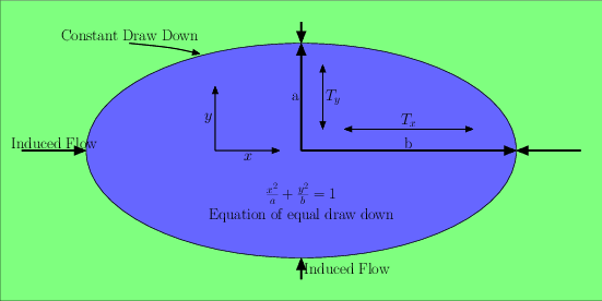
Schematic of an equal drawdown curve around a well in an anisotropic aquifer.#
Mesh#
The mesh consists of 12,208 cells. There is a single cell in the z-direction, which is uniform \(\Delta z=5.0\) m everywhere.
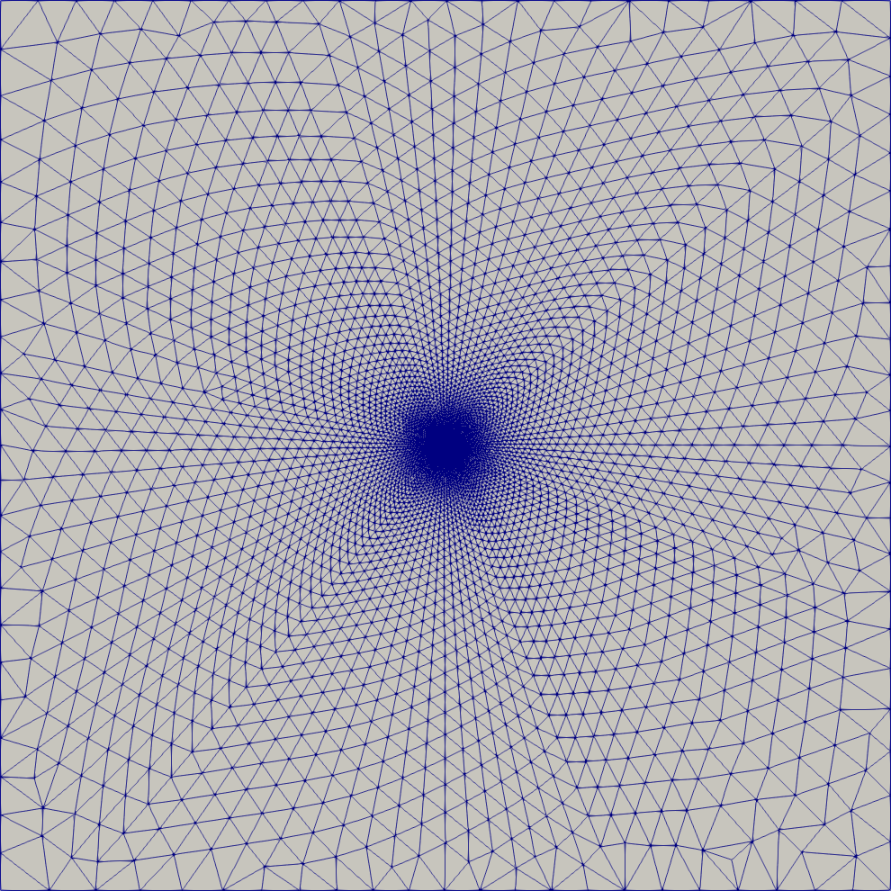
Unstructured computational mesh with 12208 cells.#
Variables#
Domain:
\(x_{min} = y_{min} = -1200\), \(z_{min} = 0 \text{ [m]}\)
\(x_{max} = y_{max} =1200\), \(z_{max} = 5 \text{ [m]}\)
aquifer thickness: \(b=z_{max}-z_{min}=5 \text{ [m]}\)
pumping well location: \((x,y) = (0,0) \text{ [m]}\), spanning entire aquifer thickness
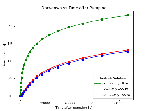
observation well locations:
\((x_{obs1},y_{obs1},z_{obs1}) = (55.0, 0.0, 2.0) \text{ [m]}\)
\((x_{obs2},y_{obs2},z_{obs2}) = (0.0, 55.0, 2.0) \text{ [m]}\)
\((x_{obs3},y_{obs3},z_{obs3}) = (55.0, 55.0, 2.0) \text{ [m]}\)
Boundary and initial conditions:
initial hydraulic head: \(h(x,y,0)=h_0 \: \text{[m]}\), where \(h_0\) is hydrostatic (i.e. drawdown \(s=0 \text{ [m]}\))
constant-head (Dirichlet) lateral boundary conditions: \(h(x_{min,max},y_{min,max},t)=h_0 \: \text{[m]}\)
no-flow (Neumann) upper and lower boundary conditions
well-head pumping rate: \(Q=2.0 \: \text{[m}^3\text{/s]}\)
duration of pumping: \(t_{max}=86400\: \text{[s]} = 1 \text{ [day]}\)
Material properties:
storativity: \(S=3.75 \times 10^{-4} \: \text{[-]}\)
derived from: \(S=S_s b\), where \(S_s=7.5 \times 10^{-5} \: \text{[m}^{-1} \text{]}\) and \(b=5 \: \text{[m]}\)
porosity: \(\phi = 0.3\)
transmissivity: \(T_x= 1.15 \times 10^{-3}, T_y= 1.15 \times 10^{-4} \: \text{[m}^2\text{/s]}\)
derived from: \(T=Kb\), where \(K=\frac{k \rho g}{\mu}\)
intrinsic permeability tensor: \(k_x = 2.3543 \times 10^{-11}, k_y = k_z = 2.3543 \times 10^{-12} \: \text{[m}^2\text{]}\)
fluid density: \(\rho = 998.2 \: \text{[kg/m}^3\text{]}\)
dynamic viscosity: \(\mu = 1.002 \times 10^{-3} \: \text{[Pa} \cdot \text{s]}\)
gravitational acceleration: \(g = 9.807 \: \text{[m/s}^2\text{]}\)
Results and Comparison#
Results are in good agreement with the analytic solution.
(Source code, png, hires.png, pdf)
References#
About#
Directory: testing/verification/flow/saturated/transient/hantush_anisotropic_2d
Authors: Alec Thomas, Konstantin Lipnikov
Maintainer: David Moulton (moulton@lanl.gov)
Input Files:
amanzi_hantush_anisotropic_2d-u.xml
Spec Version 2.3, unstructured mesh framework
Mesh: porflow4_6.exo
Analytic Solution:
Todo
Documentation:
Fix governing equation in Model to be homogeneous? [jpo]
Decide whether to keep structured run
Include info about analytic solution calculation?
convert units in Variables to be same as in Model?