
Transient Drawdown due to Pumping Wells in a Bounded Domain#
Capabilities Tested#
This two-dimensional flow problem — with a constant pumping rate in a heterogeneous confined aquifer — tests the Amanzi saturated flow process kernel. Capabilities tested include:
single-phase, two-dimensional flow
transient flow
saturated flow
constant-rate pumping wells
constant-head (Dirichlet) boundary conditions
specified volumetric flux (Neumann) boundary conditions
homogeneous isotropic porous medium
uniform mesh
For details on this test, see About.
Background#
As we see from the comparison of results from Amanzi and Butler’s solutions [BL91] [BL93], it is inevitable that the numerical solutions from the Amanzi model will not match the results from these analytical solutions at later time, because these analytical solutions were derived for the unbounded domains while in numerical simulations the domain is always bounded, compare with the Theis test. In this example, we will verify the Amanzi model using the solution for the bounded domain with uniform hydraulic properties.
Model#
Transient flow in saturated uniform porous media can be represented by
where \(h\) [L] is the head, \(t\) [T]is the time, \(T\) [L2/T] is the transmissivity, \(S\) [-] is the storage coefficient, \(Q_i\) [L3/T] is the pumpage at a well located at \((x_i,y_i)\) that starts pumping at \(t_i\), \(N_w\) is the number of pumping wells, \(\delta(x,y)\) is the Dirac delta function, being 1 for \(x = y = 0\) and 0 otherwise, and \(H(x)\) is the Heaviside function, being 1 for \(x \ge 0\) and 0 otherwise.
Initially the head is a constant everywhere in the domain:
The boundary conditions are:
where \(\Gamma_D\) is the Dirichlet boundary and \(\Gamma_N\) is the Neumann boundary.
The drawdown solution can be written as
where \(\alpha_m = m \pi/L_1, m=1,2,\cdots\), \(\beta_n = n \pi/L_2, n=0,2,\cdots\), \(L_1\) and \(L_2\) are the domain size in the x and y directions, respectively, \(D = L_1L_2\) is the area of the domain, \(a_0 =1/2\), and \(a_n =1\) for \(n \ge 1\).
Problem Specification#
Schematic#
The domain configuration and well locations are indicated in the following schematic.
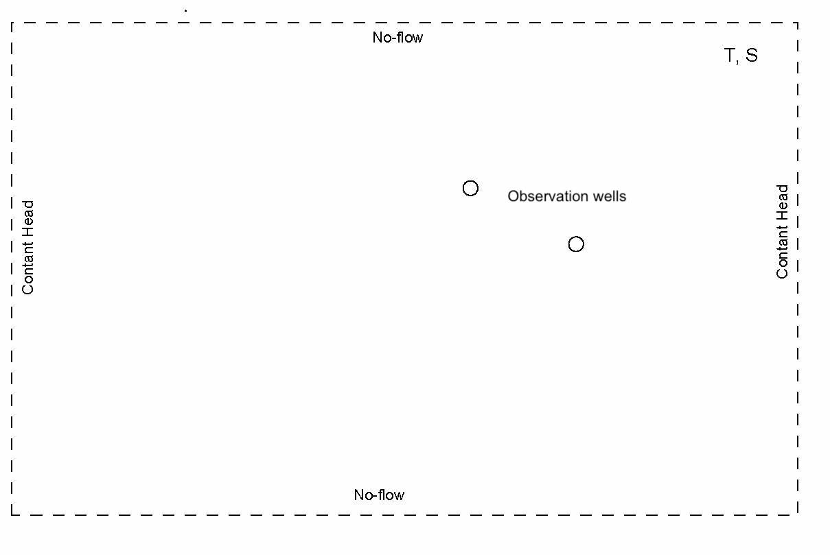
Schematic of verification problem for bounded domains.#
Mesh#
The model domain is 2400 m \(\times\) 2400 m. It has 3600 grid cells: 600 cells in the x-direction, 600 cells in y-direction, and 1 cell in the z-direction.
Variables#
Domain:
pumping well coordinates: \((x_i,y_i) = (1200 \text{ m}, 1200 \text{ m})\)
observation well coordinates: \((1224 \text{ m}, 1200 \text{ m})\) and \((1300 \text{ m}, 1200 \text{ m})\)
respective distances from pumping well: \(24 \text{ m}\) and \(100 \text{ m}\)
Boundary and initial conditions:
initial hydraulic head: \(h(r,0)=100.0 \: \text{[m]}\)
derived from: \(p-p_0 = \rho gh\), where reference pressure \(p_0\) is at \(z=10 \text{ [m]}\) and \(p=1.07785 \times 10^6 \text{ [Pa]}\)
constant-head (Dirichlet) far-field lateral (east, west) boundary conditions: \(h(x_{max},t)=h(y_{max},t)=100.0 \: \text{[m]}\)
no-flow (Neumann) north and south boundary conditions
well-head pumping rate: \(Q=-11.5485 \: \text{[m}^3\text{/s]}\)
Material properties:
storativity: \(S=2 \times 10^{-4} \text{ [-]}\)
derived from: \(S=S_s b\), where \(S_s=2.0 \times 10^{-4} \: \text{[m}^{-1} \text{]}\) and \(b=1 \: \text{[m]}\)
transmissivity: \(T=0.011617 \: \text{[m}^2\text{/s]}\)
derived from: \(T=Kb\), where \(K=\frac{k \rho g}{\mu}\)
intrinsic permeability: \(k = 1.187 \times 10^{-9} \: \text{[m}^2\text{]}\)
porosity: \(\phi = 0.25\)
fluid density: \(\rho = 1000.0 \: \text{[kg/m}^3\text{]}\)
dynamic viscosity: \(\mu = 1.002 \times 10^{-3} \: \text{[Pa} \cdot \text{s]}\)
gravitational acceleration: \(g = 9.807 \: \text{[m/s}^2\text{]}\)
Results and Comparison#
Comparison of Analytic Solution and Amanzi Results#
(Source code, png, hires.png, pdf)
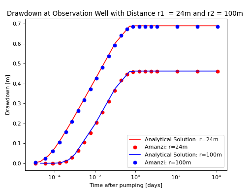
The comparison shows that the results from the Amanzi model are nearly identical to those from the analytical solution. Detailed comparison can be found in [LHB14].
References#
J. J. Butler and W. Liu. Pumping test in non-uniform aquifers – the linear strip case. J. Hydrol., 128:69–99, 1991.
J. J. Butler and W. Liu. Pumping tests in nonuniform aquifers: the radially asymmetric case. WaterResourcesResearch, 29(2):259–269, 1993.
Z. Lu, D. Harp, and K. Birdsell. Comparison of the amanzi model against analytical solutions and the fehm model. Technical Report, Los Alamos National Laboratory, Los Alamos, NM, 2014.
About#
Directory: testing/verification/flow/saturated/transient/boundedDomain
Authors: Zhiming Lu (zhiming@lanl.gov), Dylan Harp (dharp@lanl.gov)
Maintainer(s): Zhiming Lu, Dylan Harp
Input Files:
amanzi_boundedDomain_2d.xml, Spec, Version 2.3, unstructured mesh framework
Analytical Solutions
Directory: analytic/
Executable: boundedDomain.x, compiled from FORTRAN code under Linux environment.
Input Files:
Output Files:
test_h_tr.dat, drawdown as a function of time for all observation wells