
2D Dispersive Transport in a Uniform Flow Field (diagonal)#
Capabilities Tested#
This two-dimensional transport problem — with a constant rate mass loading point source in a steady-state flow field — tests the Amanzi flow process kernel as well as advection and dispersion features of the transport process kernel. It is a slight modification of the previous test (2D Dispersive Transport in a Uniform Flow Field (aligned)): the direction of the velocity field is rotated by \(45^\circ\) counter-clockwise with respect to the mesh. Thus, the test simulates non-grid-aligned advective and dispersive transport. Capabilities tested include:
single-phase, one-dimensional flow
two-dimensional transport
steady-state saturated flow
constant-rate solute mass injection well
advective transport
dispersive transport
longitudinal and transverse dispersivity
non-reactive (conservative) solute
homogeneous porous medium
isotropic porous medium
statically refined (non-uniform) mesh
For details on this test, see About.
Background#
Numerical dispersion caused by flow and transport processes not aligned with the rectangular grid can cause numerical solutions to be innacurate. Such flow and transport regimes can arise if different solutes are injected at different rates, or if the model domain is characterized by geologic media with non-uniform anisotropy, to name a couple examples. It is therefore desirable to minimize this numerical dispersion in numerical flow and transport schemes.
This test problem is a slight modification of the previous test (2D Dispersive Transport in a Uniform Flow Field (aligned)): the direction of the velocity field is rotated by \(45^\circ\) counter-clockwise with respect to the mesh.
Model#
The analytical solution addresses the advection-dispersion equation (saturation \(s_l = 1\)):
where \(\phi\) is porosity, \(C\) is the solute concentration [kg/m3], \(t\) is time [s], \(Q\) is solute mass injection rate [kg of tracer/m3/s], and \(\boldsymbol{D}\) is the dispersion tensor:
Let \(\boldsymbol{v} = (v_x,\,v_y)\) denote the pore velocity. Then, the diagonal entries in the dispersion tensor are
where \(\alpha_L\) is longitudinal dispersivity [m] and \(\alpha_T\) is transverse dispersivity [m]. The off-diagonal entries are:
Problem Specification#
Schematic#
The flow direction and source location are shown in the following schematic.

Plume from point source loading in a constant uniform groundwater flow field.#
Mesh#
The background mesh consists of square cells with size \(H=15\) m. It has 83 grid cells in the x-direction and 83 grid cells in the y-direction. The mesh is gradually refined toward the source such that the well is represented by a square cell of \(h=0.46875\) [m] (\(h = H/32\)). The mesh refinement adds 8.4% more cells.
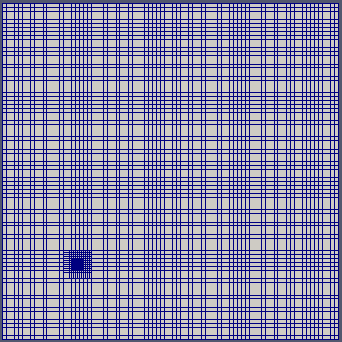
Computational mesh with 7468 cells and static refinement around the well.#
Variables#
initial concentration condition: \(C(x,0)=0 \: \text{[kg/m}^3\text{]}\)
constant solute mass injection rate: \(Q=8.1483 \times 10^{-8} \: \text{[kg/m}^3\text{/s]}\)
volumetric fluid flux: \(\boldsymbol{q}=(1.3176 \times 10^{-6},\,1.3176 \times 10^{-6}) \: \text{[m}^3 \text{/(m}^2 \text{ s)]}\) or \(\text{[m/s]}\)
Material properties:
isotropic hydraulic conductivity: \(K = 84.41 \: \text{[m/d]}\) derived from \(K=\frac{k \rho g}{\mu}\), where permeability \(k = 1.0 \times 10^{-10} \text{ [m}^2\text{]}\)
porosity: \(\phi=0.35\)
longitudinal dispersivity: \(\alpha_L=21.3 \: \text{[m]}\)
transverse dispersivity: \(\alpha_T=4.3 \: \text{[m]}\)
fluid density: \(\rho = 998.2 \: \text{[kg/m}^3\text{]}\)
dynamic viscosity: \(\mu = 1.002 \times 10^{-3} \: \text{[Pa} \cdot \text{s]}\)
gravitational acceleration: \(g = 9.807 \: \text{[m/s}^2\text{]}\)
total simulation time: \(t=1400 \: \text{[d]}\)
Results and Comparison#
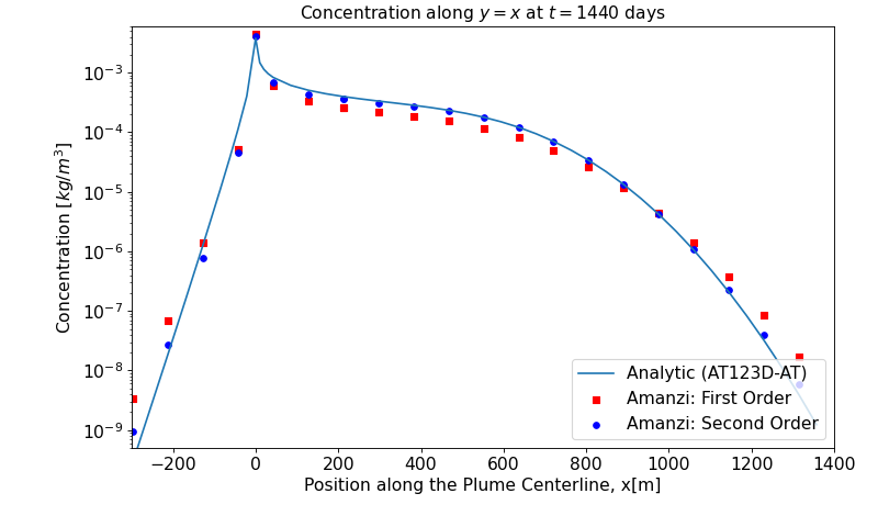
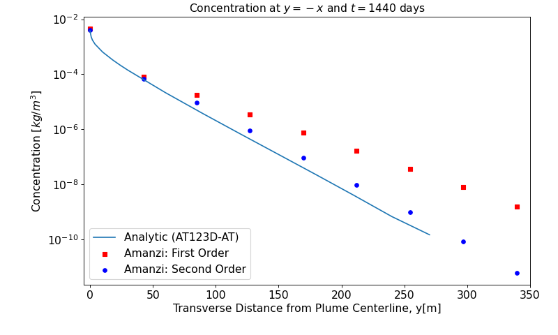
The plume structure is characterized by three line cuts. The first cut is given by line \(y=x\) that goes through the well. The two other cuts are given by tranverse cuts \(y=-x\) and \(y=\sqrt{848}-x\).
(Source code, png, hires.png, pdf)
x [m] |
Analytic (AT123D-AT) |
Amanzi First-Order |
Amanzi Second-Order |
|---|---|---|---|
-296.98 |
2.938459E-10 |
3.44205e-09 |
9.49164e-10 |
-212.13 |
1.880539E-08 |
6.94953e-08 |
2.72514e-08 |
-127.28 |
0.129059E-05 |
1.42371e-06 |
7.76863e-07 |
-42.43 |
0.113739E-03 |
5.11845e-05 |
4.61099e-05 |
0.00 |
0.377547E-02 |
4.43307e-03 |
4.27107e-03 |
42.43 |
0.833669E-03 |
6.06773e-04 |
7.02422e-04 |
127.28 |
0.508029E-03 |
3.32882e-04 |
4.29206e-04 |
212.13 |
0.397582E-03 |
2.62877e-04 |
3.56990e-04 |
212.13 |
0.397582E-03 |
2.62877e-04 |
3.56990e-04 |
296.98 |
0.333776E-03 |
2.20378e-04 |
3.08951e-04 |
381.84 |
0.284057E-03 |
1.86443e-04 |
2.68503e-04 |
466.69 |
0.234339E-03 |
1.52919e-04 |
2.25520e-04 |
551.54 |
0.179028E-03 |
1.17087e-04 |
1.74392e-04 |
636.40 |
0.121285E-03 |
8.09264e-05 |
1.19134e-04 |
721.25 |
0.702010E-04 |
4.91573e-05 |
6.92730e-05 |
806.10 |
0.338008E-04 |
2.57479e-05 |
3.34020e-05 |
890.95 |
0.132446E-04 |
1.14898e-05 |
1.31490e-05 |
975.81 |
0.417241E-05 |
4.34007e-06 |
4.19779e-06 |
1060.66 |
0.104343E-05 |
1.38453e-06 |
1.08664e-06 |
1145.51 |
0.205903E-06 |
3.73300e-07 |
2.29090e-07 |
1230.37 |
0.319697E-07 |
8.53397e-08 |
3.96315e-08 |
1315.22 |
0.387359E-08 |
1.71874e-08 |
5.76306e-09 |
The analytic data were computed with the AT123DAT software package. A difference observed near downstream boundary for the Amanzi with the first-order transport scheme (Amanzi(1st)). The second-order transport scheme provides excellent match.
(Source code, png, hires.png, pdf)
y [m] |
Analytic (AT123D-AT) |
Amanzi First-Order |
Amanzi Second-Order |
|---|---|---|---|
0.00 |
3.775286E-03 |
4.43307e-03 |
4.27107e-03 |
42.43 |
3.775286E-03 |
8.18044e-05 |
6.71725e-05 |
84.85 |
3.775286E-03 |
1.76911e-05 |
9.27840e-06 |
127.28 |
3.775286E-03 |
3.55340e-06 |
8.92789e-07 |
169.71 |
3.775286E-03 |
7.75699e-07 |
9.38170e-08 |
212.13 |
3.775286E-03 |
1.72197e-07 |
9.86303e-09 |
254.56 |
3.775286E-03 |
3.78140e-08 |
9.72459e-10 |
296.98 |
3.775286E-03 |
8.02207e-09 |
8.50556e-11 |
339.41 |
3.775286E-03 |
1.60306e-09 |
6.41251e-12 |
References#
About#
Directory: testing/verification/transport/saturated/steady-state/dispersion_45_point_2d
Author: Konstantin Lipnikov
Maintainer: David Moulton (moulton@lanl.gov)
Input Files:
amanzi_dispersion_45_point_2d-u.xml, Spec Version 2.3
mesh amanzi_dispersion_45_point_2d.exo
Analytic solution computed with AT123D-AT
Subdirectory: at123d-at
Input Files:
at123d-at_centerline.list, at123d-at_centerline.in
at123d-at_slice_x=0.in
Todo
write script to generate the tranverse cut at distance 420 m from well [jpo]
need *.list file for slice x=0? [jpo]