
Steady-State One-Dimensional Flow: Materials in Parallel#
Capabilities Tested#
This two-dimensional steady-state flow problem tests the Amanzi saturated flow process kernel. Capabilities tested include:
single-phase, one-dimensional head, two-dimentional flux
steady-state flow
saturated flow
constant-head (Dirichlet) boundary conditions
heterogeneous porous medium
isotropic porous medium
uniform mesh
For details on this test, see About.
Background#
For steady-state flow through a saturated porous medium with constant properties, the general governing differential equation expressing mass conservation and Darcy’s law [Dar56] becomes simply
(1)#\[\frac{d^2h}{dx^2} = 0\]
where the total head (\(h\), [L]) is the sum of pressure head (\(P/\rho g\), [L]) and elevation (\(z\), [L])
\[h = \frac{P}{\rho g}+z\]
\(\rho\) = density [M/L3], \(g\) = gravitational acceleration [L/T2], and \(x\) = horizontal distance [L]. The ordinary differential equation (1) is easily solved by direct integration as
(2)#\[h = C_1 x + C_2\]
where the integration constants \(C_1\) and \(C_2\) depend on the boundary conditions.
For a simple heterogeneous porous medium composed of two constant-property materials in parallel, Equation (2) can be applied to each subregion separately. To analyze this special case, let the subscripts 1 and 2 denote the two subregions.
Model#
The analytic solution for prescribed inlet and outlet pressures is shown below. When hydraulic head is prescribed at both boundaries as
(3)#\[\begin{split}h(0) &= h_0\\ h(L) &= h_L\end{split}\]
the analytic solution (3) for hydraulic head in each subregion (\(h_i\), [L]) becomes
(4)#\[h_i = (h_L - h_0) \frac{x}{L} + h_0, i=1,2\]
where \(L\) = domain length [L]. The volumetric flowrate per unit area through a porous medium, or Darcy velocity (\(U\), [L/T]), is defined by Darcy’s law as
(5)#\[U = -\frac{k}{\mu\rho g}\frac{dh}{dx} = -K\frac{dh}{dx}\]
where \(k\) = intrinsic permeability [L2], \(\mu\) = viscosity [M/LT], and \(K\) = hydraulic conductivity [L/T]. Applying Equation (5) to each subregion using Equation (4) yields
(6)#\[U_i = K_i\frac{h_0 - h_L}{L}, i=1,2\]
Note that the hydraulic head and Darcy velocity in each subregion are independent of the properties of the other subregion.
Problem Specification#
The analytic solutions for hydraulic head and Darcy velocity can be used to test Amanzi implementation of prescribed hydraulic head boundary conditions, Darcy’s law, and mass conservation on an elementary problem with discrete heterogeneity.
Schematic#
The domain is shown in the following schematic.
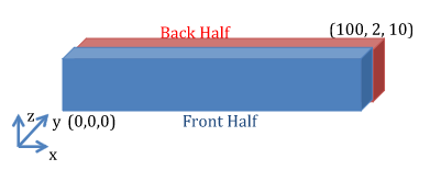
One-dimensional, steady-state flow through a saturated porous medium with constant properties#
Mesh#
A steady-flow mesh is applied. The mesh consists of 400 cells: 20 grid cells in the x-direction, 2 cells in the y-direction, and 1 cell in the z-direction. Mesh discretization is as follows: \(\Delta x = 5 \: m, \: \Delta y = 1 \: m,\) and \(\Delta z = 10 \: m\).
Variables#
To generate numerical results the following specifications are considered:
Domain
\(x_{min} = y_{min} = z_{min} = 0\)
\(x_{max} = 100 \: m, \: y_{max} = 2 \: m, \: z_{max} = 10 \: m\)
Horizontal flow in the x-coordinate direction
no-flow prescribed at the \(y_{min}, \: y_{max}, \: z_{min}, \: z_{max}\) boundaries
prescribed hydraulic head at the x-coordinate boundaries: \(h(0) = 20 \: m, \: h(L) = 19 \: m\)
Material properties:
\(\rho = 998.2 \: kg/m^3, \: \mu = 1.002 \times 10^{-3} \: Pa\cdot s, \: g = 9.807 \: m/s^2\)
\(K_1 = 1.0 \: m/d\) \((k = 1.1847 \times 10^{-12} \: m^2)\) for \(0 \: m \leqslant y \leqslant 1 \: m\)
\(K_2 = 10 \: m/d\) \((k = 1.1847 \times 10^{-11} \: m^2)\) for \(1 \: m \leqslant y \leqslant 2 \: m\)
Model discretization
\(\Delta x = 5 \: m, \Delta y = 1 \: m, \Delta z = 10 \: m\)
For these input specifications, Amanzi simulation output is expected to closely match
(7)#\[h_i = 20m -\frac{x}{100m}, \: i=1,2\]
and
(8)#\[\begin{split}U_1 &= 0.01 \: m/d\\ U_2 &= 0.1 \: m/d\end{split}\]
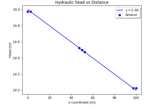
Results and Comparison#
The discretization is exact for linear solutions, and it is clear in the figure that Amanzi has reproduced the exact solution. At a boundary point, the observation is taken from a nearby cell. This will be fixed in the future.
(Source code, png, hires.png, pdf)
This is also visible in the following table. The top and bottom parts of this table corerspond to the front and back materials, respectively.
x [m] |
z [m] |
Analytic [m] |
Amanzi [m] |
0.0 |
5.0 |
20.0000 |
19.9750 |
2.5 |
5.0 |
19.9750 |
19.9750 |
47.5 |
5.0 |
19.5250 |
19.5250 |
50.0 |
5.0 |
19.5000 |
19.5000 |
52.5 |
5.0 |
19.4750 |
19.4750 |
97.5 |
5.0 |
19.0250 |
19.0250 |
100.0 |
5.0 |
19.0000 |
19.0250 |
0.0 |
5.0 |
20.0000 |
19.9750 |
2.5 |
5.0 |
19.9750 |
19.9750 |
47.5 |
5.0 |
19.5250 |
19.5250 |
50.0 |
5.0 |
19.5000 |
19.5000 |
97.5 |
5.0 |
19.0250 |
19.0250 |
52.5 |
5.0 |
19.4750 |
19.4750 |
100.0 |
5.0 |
19.0000 |
19.0250 |
References#
H. Darcy. Les fontaines publiques de la ville de Dijon: exposition et application des principes a suivre et des formules a employer. Dalmont, 1856.
About#
Directory: testing/verification/flow/saturated/steady-state/linear_materials_parallel_1d
Authors: Greg Flach
Maintainer(s): David Moulton, moulton@lanl.gov
Input Files:
amanzi_linear_materials_parallel_1d-s.xlm
Spec Version 2.3.0, structured mesh framework
mesh: steady-flow_mesh.h5
runs
amanzi_linear_materials_parallel_1d-u.xml
Spec Version 2.3.0, unstructured mesh framework
mesh: generated in file
runs
Mesh Files:
steady-flow_mesh.h5
unstructured mesh is generated in file
Analytic solution computed with golden output
Subdirectory: golden_output
Input Files:
steady-flow_data.h5
Todo
keb: List what is expected out of Amanzi simulation output.
fix observation at boundary points