
Steady-State One-Dimensional Flow: Materials in Serial#
Capabilities Tested#
This one-dimensional, steady-state test shows Amanzi’s capability to simulate flow through a saturated porous medium with constant properties. Capabilities tested include,
one-dimensional representation
steady-state
saturated flow
heterogeneous porous medium
exactness of the numerical scheme for piecewise linear head
For details on this test, see About.
Background#
For one-dimensional, steady-state, flow through a saturated porous medium with constant properties, the general governing differential equation expressing mass conservation and Darcy’s law becomes simply
(1)#\[\frac{d^2h}{dx^2} = 0\]
where the total head (\(h\), [L]) is the sum of pressure head (\(P/\rho g\), [L]) and elevation (\(z\), [L])
\[h = \frac{P}{\rho g}+z\]
\(\rho\) = density [M/L3], \(g\) = gravitational acceleration [L/T2], and \(x\) = horizontal distance [L]. The ordinary differential equation (1) is easily solved by direct integration as
(2)#\[h = C_1 x + C_2\]
where the integration constants \(C_1\) and \(C_2\) depend on the boundary conditions.
For a simple heterogeneous porous medium composed of two constant-property materials in series, Equation (2) can be applied to each subregion separately with the interface conditions treated as boundary conditions for the two subregions. To analyze this special case, let the subscripts 1 and 2 denote the subregions adjoining the \(x = 0\) and \(x = L\) boundaries respectively, and the subscript i denote the interface.
Model#
The analytic solution for prescribed inlet and outlet pressures is presented below.
When hydraulic head is prescribed at both boundaries as
(3)#\[\begin{split}h(0) &= h_0\\ h(L) &= h_L\end{split}\]
the analytic solutions (2) for hydraulic head in each subregion become
(4)#\[\begin{split}h_1 &= (h_i - h_0) \frac{x}{L_i} + h_0\\ h_2 &= (h_L - h_i) \frac{x-L_i}{L-L_i} + h_i\end{split}\]
where \(L\) = domain length [L], \(L_i\) = position of interface [L], and \(h_i\) is yet to be defined. The volumetric flowrate per unit area through a porous medium, or Darcy velocity (\(U\), [L/T]), is defined by Darcy’s law as
(5)#\[U = -\frac{k}{\mu\rho g}\frac{dh}{dx} = -K\frac{dh}{dx}\]
where \(k\) = intrinsic permeability [L2], \(\mu\) = viscosity [M/LT], and \(K\) = hydraulic conductivity [L/T]. Applying Equation (5) to each subregion using Equations (4) yields
(6)#\[\begin{split}U_1 &= K_1\frac{h_0 - h_i}{L_i}\\ U_2 &= K_2\frac{h_i - h_L}{L-L_i}\\\end{split}\]
Mass conservation at the interface implies \(U_1 = U_2\), which after some algebra leads to an expression for hydraulic head at the interface:
(7)#\[h_i = \frac{K_1(L-L_i)h_0+K_2L_ih_L}{K_1(L-L_i)+K_2L_i}\]
Equations (4) and (7) collectively define hydraulic head across the domain, and Equation (6) or (7) the Darcy velocity. One can also show that
(8)#\[U = K_h\frac{h_0 - h_L}{L}\]
where \(K_h\) is the harmonic mean
(9)#\[K_h = \frac{K_1K_2L}{K_1(L-L_i) + K_2L_i}\]
Problem Specification#
The analytic solutions for hydraulic head and Darcy velocity can be used to test Amanzi implementation of prescribed hydraulic head boundary conditions, Darcy’s law, and mass conservation on an elementary problem with discrete heterogeneity.
Schematic#
The domain is shown in the following schematic.
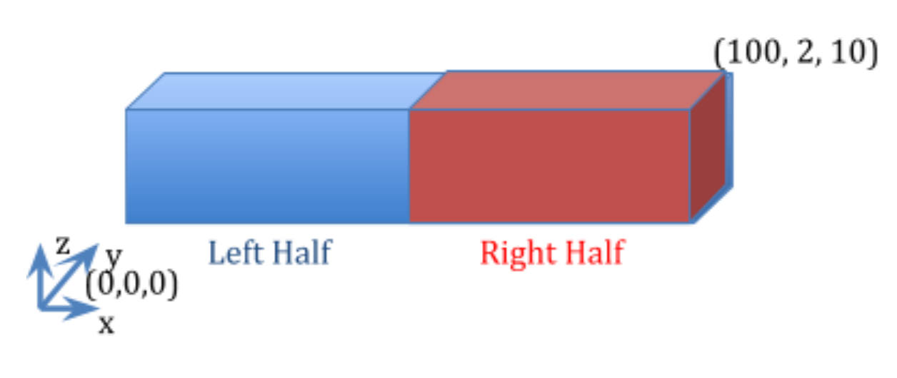
One-dimensional, steady-state flow through a saturated porous medium with constant properties.#
Mesh#
A fixed mesh with resolution 1 m is applied.
Variables#
To generate numerical results the following specifications are considered:
Domain
\(x_{min} = y_{min} = z_{min} = 0\)
\(x_{max} = 100 \: m, y_{max} = 2 \: m, z_{max} = 10 \: m\)
Horizontal flow in the x-coordinate direction
no-flow prescribed at the \(y_{min}, y_{max}, z_{min}, z_{max}\) boundaries
prescribed hydraulic head at the x-coordinate boundaries: \(h(0) = 20 \: m, h(L) = 19 \: m\)
Material properties:
\(\rho = 998.2 \: kg/m^3, \mu = 1.002 \times 10^{-3} \: Pa\cdot s, g = 9.807 \: m/s^2\)
\(L_i = x_{max}/2\)
\(K_1 = 1.0 m/d\) \((k = 1.1847 \times 10^{-12} \: m^2)\)
\(K_2 = 10 m/d\) \((k = 1.1847 \times 10^{-11} \: m^2)\)
Model discretization
\(\Delta x = \: 5 m, \Delta y = 2 \: m, \Delta z = 10 \: m\)
For these input specifications, Amanzi simulation output is expected to closely match
(10)#\[h_i = 19.090909 \:m\]
and exhibit a linear head profile within each subregion following Equations (4). The harmonic mean is \(1.818181818 \:m/d\) from Equation (9) and thus the expected Darcy velocity is
(11)#\[U = 0.0181818 \: m/d\]
from Equation (8).
Results and Comparison#
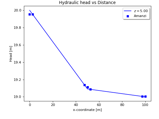
The discretization is exact for linear solutions, and it is clear in the figure that Amanzi has reproduced the exact solution inside the materials. On the boundary, the observation value is taken from the nearby cell. On the material interface, the head is averaged of head in two neighboring cells. This will be fixed in the future.
(Source code, png, hires.png, pdf)
This is also shown in the table below.
x [m] |
z [m] |
Analytic [m] |
Amanzi [m] |
0.0 |
5.0 |
20.0000 |
19.9545 |
2.5 |
5.0 |
19.9545 |
19.9545 |
47.5 |
5.0 |
19.1364 |
19.1364 |
50.0 |
5.0 |
19.0909 |
19.1114 |
52.5 |
5.0 |
19.0864 |
19.0864 |
97.5 |
5.0 |
19.0045 |
19.0045 |
100.0 |
5.0 |
19.0000 |
19.0045 |
References#
About#
Directory: testing/verification/flow/saturated/steady-state/linear_materials_serial_1d
Authors: Greg Flach
Maintainer(s): David Moulton, moulton@lanl.gov
Input Files:
amanzi_linear_materials_serial_1d-s.xlm
Spec Version 2.3.0, structured mesh framework
mesh: steady-flow_mesh.h5
runs
amanzi_linear_materials_serial_1d-u.xml
Spec Version 2.3.0, unstructured mesh framework
runs
Mesh Files:
steady-flow_mesh.h5
Analytic solution computed with golden output
Subdirectory: golden_output
Input Files:
steady-flow_data.h5
Todo
keb: List what is expected out of Amanzi simulation output.
fixed observation on the boundary and at the material interface.