
1D Conservative tracer transport#
Overview and Capabilities tested#
This test example performs the simulation of advective transport of a single conservative tracer component, testing the following capabilities:
1D flow
1D advective (single-component) transport
For details on this test, see About.
Background#
When running a reactive transport problem, it is good practice to include a non-reactive component or tracer. Results obtained for this conservative tracer can be compared to results for reactive components. This comparison can provide insights into the effects of reactions on the fate of the reactive species, e.g. retardation of species subject to sorption. The problem presented here simulates the conservative (advective) transport of a single component in a 1D domain. The flow and transport components of this test problem are used as basis to develop the following reactive transport test problems: 1D Tritium first-order decay, 1D Calcite dissolution, 1D Ion exchange.
Model#
Flow and Transport#
The flow equation solved is the saturated flow equation:
\(\frac{\partial}{\partial t} (\phi \rho) + \nabla(\rho \mathbf{q}) = 0\)
The transport equation solved is the transient advective transport equation:
\(\frac{\partial}{\partial t} (\phi c)+ \nabla(\mathbf{q} c) = 0\)
Problem Specification#
1D model domain length: 100 meters, \([x_{min},x_{max}] = [0, 100]\)
The domain is discretized with 100 cells in the x-direction, 1 meter long each.
Porosity is 0.25
The flow is horizontal in the x-direction. The uniform flow velocity in x-direction is \(7.913 \cdot 10^{-6} \text{ kg/s}\) (or \(7.927 \cdot 10^{-9} \text{ m}^3 \text{/s}\) ) specified as mass flux boundary conditions (“BC: Flux”) at the inlet end of the domain, i.e. “Inward Mass Flux” at \(x_{min} = 0 \text{ m}\) ). The oulet end of the domain ( \(x_{max} = 100 \text{ m}\) ) is assigned a “BC: Uniform Pressure” boundary condition with p = 0. The flow velocity value is chosen so that it takes 1 year for water to move 1 cell of the discretization. Flow is solved to steady state before starting the transport solve (“Initialize To Steady”).
Simulation time = 50 years
The concentration of the tracer is set to \(10^{-20} \text{ mol/Kg}\) initially everywhere in the domain. From time 0, a solution with a tracer concentration of \(10^{-3} \text{ mol/Kg}\) is injected during the entire simulation time (50 years).
Results and Comparison#
Expected results#
The flow solution is trivial and is independent of the choice of permeability. The flow velocity everywhere in the domain should be \(7.927 \cdot 10^{-9} \text{ m}^3 \text{/s}\). The advective front moves with the flow velocity. In the simulation time (50 years), the front moves half way through the domain. In the absence of diffusion, spreading of the front can be attributed to numerical dispersion added by the numerical scheme employed.
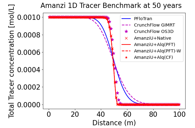
Simulation results#
In the figure below, the solution by Amanzi at time 50 years is compared to results obtained with PFloTran and CrunchFlow along the length of the domain. Amanzi, PFloTran and CrunchFlow GIMRT (the benchmark simulators used in the example) add a moderate amount of numerical dispersion to the solution. The TVD scheme used in CrunchFlow OS3D does a good job in minimizing numerical dispersion.
(Source code, png, hires.png, pdf)
About#
Benchmark simulators: PFlotran, CrunchFlow
Files:
Amanzi input file: amanzi-u-1d-tracer.xml
Benchmark simulator input file:
PFloTran: 1d-tracer.in, pflotran/1d-tracer.h5
CrunchFlow: ../calcite_1d/calcite_1d_CF.in, crunchflow/gimrt/, crunchflow/os/
Location: testing/benchmarking/chemistry/tracer_1d
Author: B. Andre, G. Hammond
Testing and Documentation: S. Molins