
1D Sorption Isotherms#
Overview and Capabilities tested#
This test example performs the simulation of sorption of aqueous components on a surface in a 1D flow domain, testing the following capabilities:
1D flow
1D advective transport
Geochemical reactions
Sorption isotherms (linear or Kd-approach, Freundlich and Langmuir)
For details on this test, see About.
Background#
The simplest model to describe sorption of a component on a surface is to relate the sorbed concentration on the surface to the concentration in the solution, thereby neglecting any additional effects on the sorption processes. Different models are available for the form of the relationship between aqueous and sorbed concentrations: the linear isotherm (or Kd-approach), the Freundlich isotherm and the Langmuir isotherm. This test example simply considers three generic components, each of which sorbs to a surface according to one isotherm model.
Model#
Flow and transport#
See the 1D Conservative tracer transport example.
Primary species#
Three generic component species are used: \(\ce{A}\), \(\ce{B}\), and \(\ce{C}\).
Isotherms#
A different sorption of isotherm is consider for each component. With each isotherm model, the sorbed concentration (\(C_s\)) is a function of the aqueous concentration of the component (\(C_{aq}\)):
The sorbed concentration of component \(\ce{A}\) is calculated according to a linear isotherm (or Kd-approach):
The sorbed concentration of component \(\ce{B}\) is calculated according to a Langmuir isotherm:
The sorbed concentration of component \(\ce{C}\) is calculated according to a Freundlich isotherm:
Problem specifications#
Flow and transport#
See the 1D Conservative tracer transport example. In this example, a solution that contains the three components at the same concentration is injected at the left boundary. As they flow down gradient they sorb according the difference sorption isotherms. The simulation is run to 50 years.
Geochemistry#
The initial concentration of the component in the domain is zero, while in the infiltrating solution their concentration is \(C_{aq}^A=C_{aq}^B=C_{aq}^C= 10^{-3} \text{mol/L}\).
The isotherm equation parameters are:
Linear isotherm: \(K_D=10\).
Langmuir isotherm: \(K=30\) and \(b=0.1\).
Freundlich isotherm: \(K_D=1.5\) and \(n=0.8\).
Results and Comparison#
Simulation results#
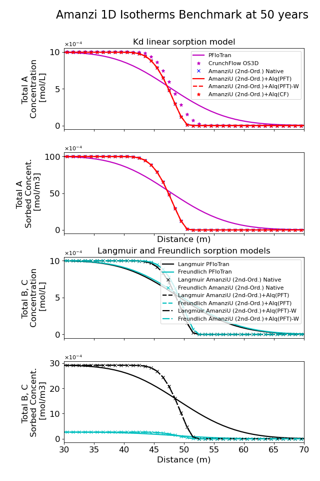
The figure below shows both the aqueous and sorbed concentrations of \(\ce{A}, \ce{B}\) and \(\ce{C}\) along the flow direction at 50 years between \(x=30 m\) and \(x=70 m\). Even though the infiltrating concentrations of the aqueous components are the same, the different models lead to different sorbed concentrations. Comparison to PFloTran results is hampered by the different numerical dispersion caused by the discretization schemes. However, the differences between isotherm model results show the same pattern as far as aqueous concentrations goes and the results in terms of sorbed concentrations are within close agreement.
(Source code, png, hires.png, pdf)
About#
Benchmark simulator: PFlotran
Files:
Amanzi input file/s (native chemistry): amanzi-u-1d-isotherms.xml
Amanzi input file/s (Alquimia chemistry): amanzi-1d-isotherms-alq.xml, 1d-isotherms.in, isotherms.dat
Benchmark simulator input file: 1d-isotherms.in, isotherms.dat
Location: testing/benchmarking/chemistry/isotherms_1d
Author: B. Andre, G. Hammond
Testing and Documentation: S. Molins
Last tested on Nov 13, 2013