
1D Calcite dissolution#
Overview and Capabilities tested#
This test example performs the simulation of calcite dissolution in a 1D flow domain, testing the following capabilities:
1D flow
1D advective transport
Geochemical reactions
Aqueous complexation reactions (equilibrium)
Mineral dissolution
For details on this test, see About.
Background#
Carbonate minerals are present in many subsurface environments and contribute to their buffering capacity. Under common subsurface flow conditons, calcite dissolution is a relatively fast geochemical reaction leading often to local geochemical equilibrium and sharp dissolution fronts. Calcite dissolution is represented here with a kinetic rate expression based on the transition state theory. In this test example, a solution under saturated with calcite is injected at x=0 into a 100-m porous domain containing calcite; as a result, calcite dissolves raising the pH and the concentration of Ca in the effluent end of the domain.
Model#
Flow and transport#
See the 1D Conservative tracer transport example.
Aqueous complexation#
Six reactions equilibrium reactions are considered in aqueous phase (by convention, secondary species are given in the left hand side, while primary species are in the right hand side):
\(\ce{OH^- <=> H2O - H^+}\), \(\text{ } \log(K)=13.9951\)
\(\ce{CO3^{--} <=> -H^+ + HCO3^-}\), \(\text{ } \log(K)=10.3288\)
\(\ce{CO2_{(aq)} <=> - H2O + H^+ + HCO3^-}\), \(\text{ } \log(K)=-6.3447\)
\(\ce{CaOH_+ <=> H2O - H^+ + Ca^{++}}\), \(\text{ } log(K)=12.85000\),
\(\ce{CaHCO3^+ <=> HCO3^- + Ca^{++}}\), \(\text{ } \log(K)=-1.0467\)
\(\ce{CaCO3_{(aq)} <=> - H^+ + HCO3^- + Ca^{++}}\), \(\text{ } \log(K)=7.0017\)
Calcite dissolution#
Calcite dissolution can be expressed as
\(CaCO_3(s) \rightarrow Ca^{2+} + CO_3^{2-}\)
The rate expression is
\(r = S \cdot k \cdot (1 - \frac{Q}{K_{sp}})\)
where \(S\) is the reactive surface area, \(k\) is the intrinsic rate constant, \(Q\) is the ion activity product, and \(K_{sp}\) is the solubility constant of calcite.
Problem Specification#
Flow and transport#
See the 1D Conservative tracer transport example. In this example, a solution at pH 5, out of equilibrium with respect to calcite, is injected at the left boundary causing calcite dissolution in the domain as it flows down gradient a 1D flow domain. The simulation is run to 50 years.
Geochemistry#
Infiltration Solution:
\(pH = 5.0\)
\(u_{\ce{HCO3^-}}=1.0028 \cdot 10^{-3} \text{ mol/Kg}\)
\(u_{\ce{Ca^{++}}}=1.684 \cdot 10^{-5} \text{ mol/Kg}\)
Solution initially in the domain:
\(pH = 8.0184\)
\(u_{\ce{HCO3^-}}=1.7398 \cdot 10^{-3} \text{ mol/Kg}\)
\(u_{\ce{Ca^{++}}}=5.2461 \cdot 10^{-4} \text{ mol/Kg}\)
Initial calcite volume fraction:
\(V_m(Calcite) = 10^{-5} \text{ m}^3 \text{ mineral/m}^3 \text{ bulk}\)
Calcite mineral surface area:
\(S = 100 \text{ m}^2 \text{/m}^3 = 1 \text{ cm}^2 \text{/cm}^3\)
Intrinsic rate constant for calcite dissolution:
\(k = 10^{-9} \text{ mol/m}^2 \text{s} = 10^{-13} \text{ mol/cm}^2 \text{s}\)
Calcite solubility:
\(\text{log}(K_{sp}) = 1.8487\)
Results and Comparison#
Expected results#
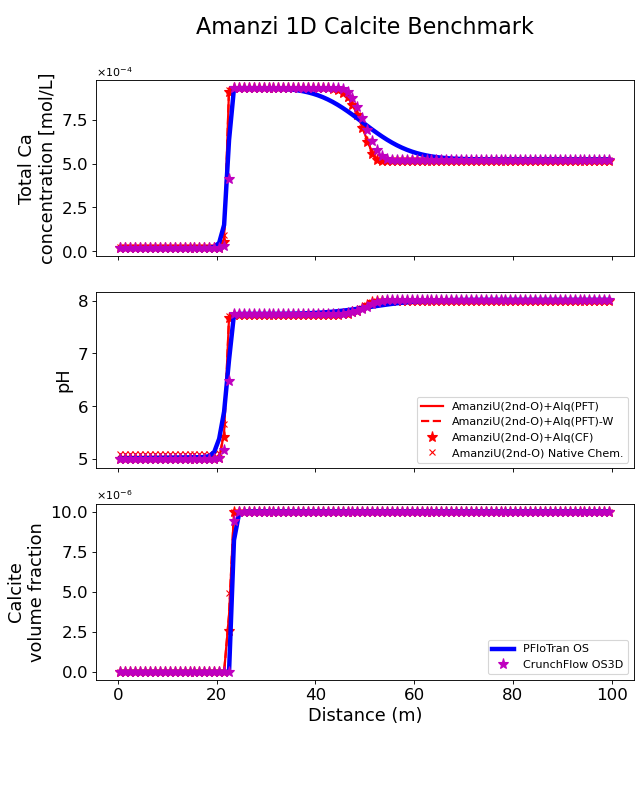
A solution with pH 5 infiltrating from the left of the domain displaces the initial solution (pH 8) and drives dissolution of calcite. Because the dissolution is relatively fast the geochemical front is sharp. In other words, as long as calcite is present the solution is near equilibrium conditions with respect to calcite. The movement of the front is dictated by how much calcite is in the domain initially (as shown by the volume fraction of calcite in the domain). Therefore, a lag is observed between the conservative tracer front and the dissolution front (see 1D Conservative tracer transport). At the dissolution a sharp increase in calcium concentration (above background levels) and a sharp increase of pH are observed, leading to near equilibrium conditions.
Simulation results#
The figure shows the concentration of total calcium, pH and Calcite volume fraction along the length of the column at the end of the simulation at 10, 20, 30, 40 and 50 years for Amanzi (run with native geochemistry and, if enabled, using the the Alquimia API with PFloTran as geochemical engine), PFloTran and CrunchFlow. PFloTran and CrunchFlow are run using the a global implicit approach and an operator splitting approach. The reader should note that CrunchFlow OS3D employs a TVD scheme for advection that minimizes numerical dispersion. A good agreement is observed between the codes. Some differences are attributable to the numerical dispersion added in the code using implicit methods for advective fluxes. Additional, differences are attributable to the implementation of the boundary conditions in the different codes.
(Source code, png, hires.png, pdf)
About#
Benchmark simulators: PFlotran, CrunchFlow
Files
Amanzi input file/s (native chemistry): amanzi-1d-calcite.xml
Amanzi input file/s (Alquimia chemistry): amanzi-1d-calcite-alq.xml, 1d-calcite.in, calcite.dat
Benchmark simulator input and output file/s:
PFloTran: 1d-calcite.in, calcite.dat, pflotran/1d-calcite.h5, pflotran/os/1d-calcite.h5
CrunchFlow: crunchflow/calcite_1d_CF.in, crunchflow/calcite_1d_CF.dbs, crunchflow/gimrt/, crunchflow/os3d/
Location: testing/benchmark/chemistry/calcite_1d/
Author: B. Andre, G. Hammond
Testing and Documentation: S. Molins
Last tested on: Oct 3, 2013